PSYC 3210 :: Laboratory Exercise - Rate Coding of Sensory Inputs

Objective

Record extracellular spiking activity from a cockroach leg in response to different stimulus intensities

Introduction

Physiology is the study of how cells, tissues, and organs function within larger systems and respond to external events. Neurophysiology is the study of how neurons function within the brain to process events in the environment and produce behaviors in response. Sensory events, neural activity, and behavior are all dynamic, and neurophysiologists need to be able to record those dynamics to study how they relate to each other. Fortunately, as neurons perform their function, they generate electrical signals that can be detected with sensitive instruments.

We will be using a classical method for detecting and recording neural activity that involves sensing and amplifying tiny electrical signals created by outside cells when they generate action potentials. You should all be familiar with how action potentials are generated, but for a refresher you can work through this series of videos from the Howard Hughes Medical Institute.

In this exercise, you will be making extracellular recordings from a cockroach leg, and learning how to measure the spikes caused by different stimuli. Once you can detect spikes, you are ready to record, quantify, and graphically present electrophysiology data. The method you will use to compare differences in spiking from different stimuli is called rate coding and it is one of the most reliable tools in neuroscience. Rate coding is simply measuring the number of spikes that occur during a set period of time. However, even though it is simple, rate coding can be used to answer complex questions about how neurons respond to stimuli.

Setup

The extracellular potentials generated by neural action potentials are very small (microvolts), and the currents they can induce in a recording electrode are also very small. We will use amplifiers from Backyard Brains to increase the power of the signals so that you can hear them and record them using a computer or smartphone.

Before class

1. Download and install the Backyard Brains app. You can use the version the runs on a PC or iOS device. Both versions are similar, but in our experience the PC version seems to have less noise (when run on a laptop) and is somewhat easier to use.

Equipment setup and surgical prep

1. Connect the spikerbox to your computer or smartphone using the audio cable. Use the black, standard cable for PCs with dedicated microphone ports; use the green smartphone cable for smartphones and PCs that have a shared microphone/headphones port (some Macbook Pros and Macbook Airs). Start the recording app, turn on the spikerbox, and verify that you can see a signal. It will just look like noise. If you don’t see anything, make sure the microphone is unmuted and that noise cancellation and dynamic gain are turned off. Ask a TA or the instructor for help if the signal is just a flat line. Unplug the cable from the spikerbox and turn it off.
2. Take a cockroach and either put it in ice water or a standard freezer to anesthetize it. Wait 5-10 minutes, or until the cockroach stops moving. Take care to monitor how long the cockroach has been placed in the water or freezer, as extended exposure to low temperatures can be fatal.
3. Once your cockroach has been anesthetized, remove it from the water or freezer and place it on your lab bench. Using dissection scissors cut off one of the mesothoracic legs (see below). Make sure you cut close to the thorax (body) so that the coxa remains attached.
4. In the space provided below, sketch your cockroach and the leg you have removed. Note any damaged parts if applicable.

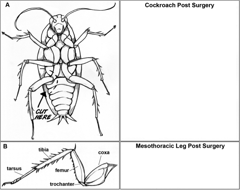
1. Return your cockroach to its housing. The leg will grow back if the cockroach is not a full-grown adult yet. One way to distinguish the age of your cockroach is to note whether the wings are fully formed. Adults have wings while younger nymphs do not.
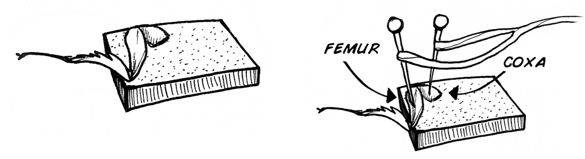
2. Place the leg on the cork found on top of your SpikerBox. Make sure the coxa and femur of the leg are on the cork, while the tibia and tarsus hang freely (below) Insert the electrodes through the leg and into the cork. Insert one electrode into the coxa and the second electrode into the femur (below). The electrodes will measure action potentials as well as keep your leg in place.

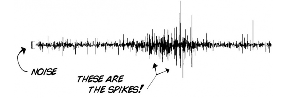
Turn your SpikerBox on! If you hear a popcorn sound, congratulations, you have just heard your first neuron firing! If you are not sure whether you are listening to spikes or noise, lightly touch spines located on the tibia with a toothpick. If you don’t hear spikes in response to toothpick stimulations, try reinserting your electrodes, switching which one is in the coxa and femur. Once you are hearing spikes consistently, plug the cable back into the spikerbox. You should see spikes that look something like this:

Recording spikes from the femur and tibia

1. Take a few moments to familiarize yourself with the recording app. Clicking and dragging in various places will change the offset and scale of the trace. The red button in the top right will start and stop a recording, saving the data to a different file each time it’s pressed. Decide if you want to start separate recordings for each stimulus condition you test, or just make one long recording. Either way, you’ll need to make notes of what files or times correspond to different conditions.
2. Try blowing on the cockroach leg or touching it with a toothpick. You should see an increase in activity, hopefully with some very sharp peaks. These correspond to individual action potentials. You’ll also note that there is noise constantly in the background. The ratio of the spike peak height to the noise is called the signal to noise ratio, and you want this to be as large as possible. To reduce noise, turn off your cell phone and Wi-Fi. Signal interference from these devices is significant. To demonstrate the importance, send a text to another phone in the same room while you are recording from the leg and listen/look for the interference in your recording. What does this tell you about how cell phones work? To increase signal, you can try repositioning the electrodes in different parts of the femur. These electrodes are pretty crude, though, so there’s a limit to how good you can get.
3. Create a table like the one below in Excel or the spreadsheet application of your choice. Record the spontaneous spiking patterns from the leg for a couple of minutes. Note the beginning and end time of recordings (for this first recording, your stimulation method will be ‘none’).
4. Take a toothpick and stimulate the barbs on the tibia of the leg. Try several variations of stimulation including constant pressure or repetitive poking, until you find one that gives you consistent reactions. Write your stimulation methods in the table.

Stimulation Method	Start	Stop	Observations
None

Now you will do a controlled experiment to see how different strengths of stimulation affect the cockroach leg. You will use compressed air on your lab bench to stimulate the cockroach leg for this experiment, varying the distance from the preparation to control the stimulus intensity. Use the provided tape measures to find the correct distances.

In each trial, you will record 30 seconds of spontaneous activity (without blowing), then about 30-60 seconds of stimulus. Be sure to note the start and stop time of the stimulus relative to the start of the recording. Repeat each stimulus condition 4 times.

Trial	Distance	Start	Stop	Observations
1	4 cm
2	6 cm
3	8 cm
4	10 cm
5	12 cm
6	4 cm
7	(add lines as needed)

Remove the electrode from the femur and move it to the tibia, as shown in the diagram.

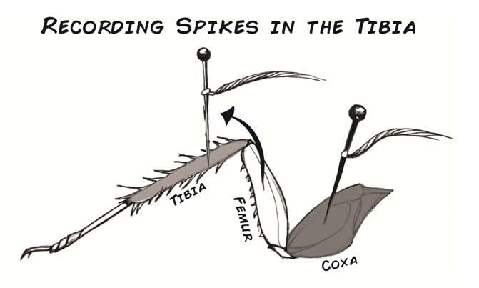
Repeat the same series of measurements that you made in the femur and record them in a table like the one above.

Data Analysis

The first step is to isolate your spikes. Begin with the file for your first 4 cm trial, then repeat the procedure for each of the other trials.

Open the file and zoom in to a representative region of your control period (with no stimulus). Continue to zoom in until you can see individual spikes. They may look something like this:

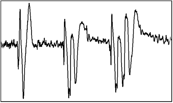
As in the example, not all your spikes may look the same. This happens for several reasons. One is that background noise produces random distortions in the spike shapes; another is that spikes are sometimes emitted as groups or bursts; and a third is that you are probably recording from more than one neuron at once, and there are differences in the shapes of the waveforms that the electrode picks up. In some experiments, people will take care to isolate a single neuron, or unit, but in many cases (including this one), the average activity from multiple neurons is enough.

Click the button at the top left that look like a flask. You will notice that this adds two controls to the right of the trace that can be dragged up and down. Adjust them so that the lower trace is above the background noise and the upper trace is above the peaks of the spikes. This configures an algorithm that will detect spikes in the recording. Save the detected spikes by clicking the disk icon. Click the flask again to go back to the recording. You should see marks above the trace that indicate where the spikes were detected. This is an example of a raster plot.

You now need to count the number of spikes that were evoked during the baseline and the stimulus period. Click and drag with the right mouse button to select around 10 s of baseline for analysis. The screen will show the duration of your analysis window, the number of spikes, and the RMS. Make a note of all three in the table below. Now select the interval when you presented a stimulus and note the same quantities. Repeat this analysis for all the recordings you made; note that you will be making two entries per trial, one for the baseline and one for the stimulus.

Trial	Location	Stimulus	Duration	Spike Count	RMS
1	femur	none
1	femur	2 cm
2	femur	none
2	femur	4 cm

Create two graphs like the ones below by hand or using your spreadsheet program to show the average spike rate as a function of stimulus intensity in the two locations you recorded, indicating the standard errors of your averages with error bars. Think carefully about what will go on the x and y axes.

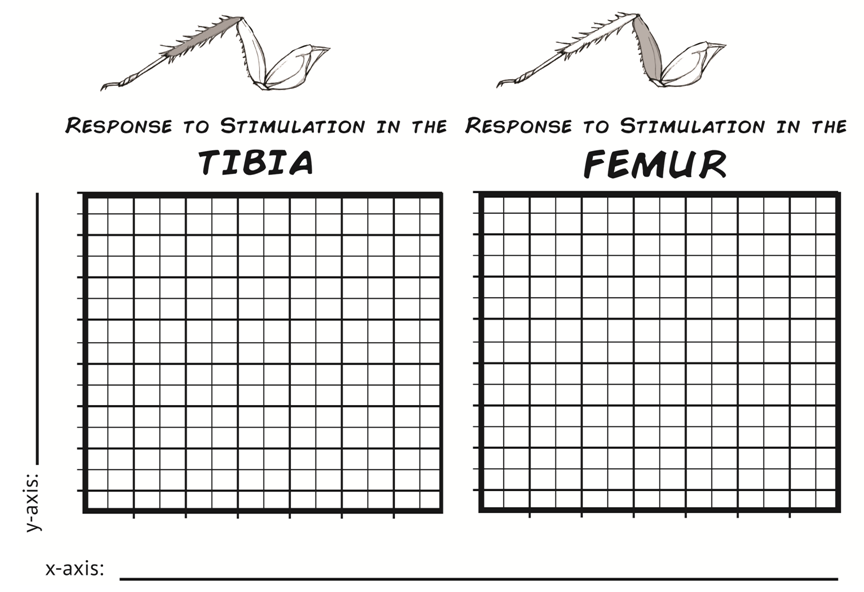
Try plotting RMS in the same way. Is RMS a good approximation of spike rate?

Discussion Questions

If time allows, discuss the following questions with your partner and/or neighboring groups:

1. During data analysis you chose a threshold for which spikes you would count. How, if at all, do you think that your results would differ if you had used a higher threshold? A lower threshold?
2. How did the neuron firing change as you stimulated the femur with increased air pressure? How did neuron firing change when you stimulated the tibia with increased air pressure?
3. Did neuron firing change when you applied the same stimulus continuously? If it did, why might this be the case?
4. What kinds of information about the stimulus were present in the neural responses you recorded?

Homework

Submit a document with your tables, graphs, and an answer to one of the discussion questions by the beginning of class next week. Make sure you save the recordings and analysis files you made! We will be using them next week.

Acknowledgments

This activity is based on activities developed by Backyard Brains. Protected under the Creative Commons License: